import matplotlib.pyplot as plt
import matplotlib as mpl
import numpy as np
import sympy as sy

sy.init_printing()
plt.style.use("ggplot")np.set_printoptions(precision=3)
np.set_printoptions(suppress=True)An eigenvector of an \(n \times n\) matrix \(A\) is a nonzero vector \(x\) such that \(Ax = \lambda x\) for some scalar \(\lambda\). A scalar \(\lambda\) is called an eigenvalue of \(A\) if there is a nontrivial solution \(x\) of \(Ax = \lambda x\), such an \(x\) is called an eigenvector corresponding to \(\lambda\).
Rewrite the equation,
\[ (A-\lambda I)x = 0 \]
Since the eigenvector should be a nonzero vector, which means:
- The column or rows of \((A-\lambda I)\) are linearly dependent
- \((A-\lambda I)\) is not full rank, \(Rank(A)<n\).
- \((A-\lambda I)\) is not invertible.
- \(\text{det}(A-\lambda I)=0\), which is called characteristic equation.
Consider a matrix \(A\)
\[ A = \begin{bmatrix} 1 & 0 & 0 \\ 1 & 0 & 1 \\ 2 & -2 & 3 \end{bmatrix} \]
Set up the characteristic equation,
\[ \text{det}\left( \begin{bmatrix} 1 & 0 & 0 \\ 1 & 0 & 1 \\ 2 & -2 & 3 \end{bmatrix} - \lambda \begin{bmatrix} 1 & 0 & 0 \\ 0 & 1 & 0 \\ 0 & 0 & 1 \end{bmatrix} \right) = 0 \]
Use SymPy charpoly and factor, we can have straightforward solutions for eigenvalues.
lamda = sy.symbols(
    "lamda"
)  # 'lamda' withtout 'b' is reserved for SymPy, lambda is reserved for Python
charpoly returns characteristic equation.
A = sy.Matrix([[1, 0, 0], [1, 0, 1], [2, -2, 3]])
p = A.charpoly(lamda)
p
\(\displaystyle \operatorname{PurePoly}{\left( \lambda^{3} - 4 \lambda^{2} + 5 \lambda - 2, \lambda, domain=\mathbb{Z} \right)}\)
Factor the polynomial such that we can see the solution.
sy.factor(p)\(\displaystyle \operatorname{PurePoly}{\left( \lambda^{3} - 4 \lambda^{2} + 5 \lambda - 2, \lambda, domain=\mathbb{Z} \right)}\)
From the factored characteristic polynomial, we get the eigenvalue, and \(\lambda =1\) has algebraic multiplicity of \(2\), because there are two \((\lambda-1)\). If not factored, we can use solve instead.
sy.solve(p, lamda)\(\displaystyle \left[ 1, \ 2\right]\)
Or use eigenvals directly.
A.eigenvals()\(\displaystyle \left\{ 1 : 2, \ 2 : 1\right\}\)
To find the eigenvector corresponding to \(\lambda\), we substitute the eigenvalues back into \((A-\lambda I)x=0\) and solve it. Construct augmented matrix with \(\lambda =1\) and perform rref.
(A - 1 * sy.eye(3)).row_join(sy.zeros(3, 1)).rref()\(\displaystyle \left( \left[\begin{matrix}1 & -1 & 1 & 0\\0 & 0 & 0 & 0\\0 & 0 & 0 & 0\end{matrix}\right], \ \left( 0,\right)\right)\)
The null space is the solution set of the linear system.
\[ \left[ \begin{matrix} x_1 \\ x_2 \\ x_3 \end{matrix} \right]= \left[ \begin{matrix} x_2-x_3 \\ x_2 \\ x_3 \end{matrix} \right]= x_2\left[ \begin{matrix} 1 \\ 1 \\ 0 \end{matrix} \right] +x_3\left[ \begin{matrix} -1 \\ 0 \\ 1 \end{matrix} \right] \]
This is called eigenspace for \(\lambda = 1\), which is a subspace in \(\mathbb{R}^3\). All eigenvectors are inside the eigenspace.
We can proceed with \(\lambda = 2\) as well.
(A - 2 * sy.eye(3)).row_join(sy.zeros(3, 1)).rref()\(\displaystyle \left( \left[\begin{matrix}1 & 0 & 0 & 0\\0 & 1 & - \frac{1}{2} & 0\\0 & 0 & 0 & 0\end{matrix}\right], \ \left( 0, \ 1\right)\right)\)
The null space is the solution set of the linear system.
\[ \left[ \begin{matrix} x_1 \\ x_2 \\ x_3 \end{matrix} \right]= \left[ \begin{matrix} 0\\ \frac{1}{2}x_3\\ x_3 \end{matrix} \right]= x_3\left[ \begin{matrix} 0 \\ \frac{1}{2} \\ 1 \end{matrix} \right] \]
To avoid troubles of solving back and forth, SymPy has eigenvects to calcuate eigenvalues and eigenspaces (basis of eigenspace).
eig = A.eigenvects()
eig
\(\displaystyle \left[ \left( 1, \ 2, \ \left[ \left[\begin{matrix}1\\1\\0\end{matrix}\right], \ \left[\begin{matrix}-1\\0\\1\end{matrix}\right]\right]\right), \ \left( 2, \ 1, \ \left[ \left[\begin{matrix}0\\\frac{1}{2}\\1\end{matrix}\right]\right]\right)\right]\)
To clarify what we just get, write
print(
    "Eigenvalue = {0}, Multiplicity = {1}, Eigenspace = {2}".format(
        eig[0][0], eig[0][1], eig[0][2]
    )
)
Eigenvalue = 1, Multiplicity = 2, Eigenspace = [Matrix([
[1],
[1],
[0]]), Matrix([
[-1],
[ 0],
[ 1]])]print(
"Eigenvalue = {0}, Multiplicity = {1}, Eigenspace = {2}".format(
eig[1][0], eig[1][1], eig[1][2]
)
)Eigenvalue = 2, Multiplicity = 1, Eigenspace = [Matrix([
[ 0],
[1/2],
[ 1]])]NumPy Functions for Eigenvalues and Eigenspace
Convert SymPy matrix into NumPy float array.
A = np.array(A).astype(float)
A
array([[ 1., 0., 0.],
[ 1., 0., 1.],
[ 2., -2., 3.]]).eigvals() and .eig(A) are handy functions for eigenvalues and eigenvectors.
np.linalg.eigvals(A)array([2., 1., 1.])np.linalg.eig(A) # return both eigenvalues and eigenvectorsEigResult(eigenvalues=array([2., 1., 1.]), eigenvectors=array([[ 0. , 0. , 0.408],
[ 0.447, 0.707, -0.408],
[ 0.894, 0.707, -0.816]]))An Example
Consider a matrix \(A\)
A = sy.Matrix(
    [
        [-4, -4, 20, -8, -1],
        [14, 12, 46, 18, 2],
        [6, 4, -18, 8, 1],
        [11, 7, -37, 17, 2],
        [18, 12, -60, 24, 5],
    ]
)
A
\(\displaystyle \left[\begin{matrix}-4 & -4 & 20 & -8 & -1\\14 & 12 & 46 & 18 & 2\\6 & 4 & -18 & 8 & 1\\11 & 7 & -37 & 17 & 2\\18 & 12 & -60 & 24 & 5\end{matrix}\right]\)
Find eigenvalues.
eig = A.eigenvals()
eig
\(\displaystyle \left\{ 2 : 2, \ 3 : 1, \ \frac{5}{2} - \frac{\sqrt{1473}}{2} : 1, \ \frac{5}{2} + \frac{\sqrt{1473}}{2} : 1\right\}\)
Or use NumPy functions, show the eigenvalues.
A = np.array(A)
A = A.astype(float)
eigval, eigvec = np.linalg.eig(A)
eigval
array([ 21.69, -16.69, 3. , 2. , 2. ])And corresponding eigenvectors.
eigvecarray([[-0.124, -0.224, 0. , -0.039, 0.611],
[ 0.886, -0.543, -0.894, -0.216, -0.149],
[ 0.124, 0.224, 0. , 0. , -0. ],
[ 0.216, 0.392, 0.447, 0.255, -0.462],
[ 0.371, 0.672, -0. , -0.942, 0.625]])A Visualization Example
Let
\[ A= \left[ \begin{matrix} 1 & 6\\ 5 & 2 \end{matrix} \right] \]
find the eigenvalues and vectors, then visualize in \(\mathbb{R}^2\)
Use characteristic equation \(|A - \lambda I|=0\)
\[ \left| \left[ \begin{matrix} 1 & 6\\ 5 & 2 \end{matrix} \right] - \left[ \begin{matrix} \lambda & 0\\ 0 & \lambda \end{matrix} \right]\right|=0 \]
lamda = sy.symbols("lamda")
A = sy.Matrix([[1, 6], [5, 2]])
I = sy.eye(2)
A - lamda * I\(\displaystyle \left[\begin{matrix}1 - \lambda & 6\\5 & 2 - \lambda\end{matrix}\right]\)
p = A.charpoly(lamda)
p
\(\displaystyle \operatorname{PurePoly}{\left( \lambda^{2} - 3 \lambda - 28, \lambda, domain=\mathbb{Z} \right)}\)
sy.factor(p)\(\displaystyle \operatorname{PurePoly}{\left( \lambda^{2} - 3 \lambda - 28, \lambda, domain=\mathbb{Z} \right)}\)
There are two eigenvalues: \(7\) and \(4\). Next we calculate eigenvectors.
(A - 7 * sy.eye(2)).row_join(sy.zeros(2, 1)).rref()\(\displaystyle \left( \left[\begin{matrix}1 & -1 & 0\\0 & 0 & 0\end{matrix}\right], \ \left( 0,\right)\right)\)
The eigenspace for \(\lambda = 7\) is
\[ \left[ \begin{matrix} x_1\\ x_2 \end{matrix} \right]= x_2\left[ \begin{matrix} 1\\ 1 \end{matrix} \right] \]
Any vector is eigenspace as long as \(x \neq 0\) is an eigenvector. Let’s find out eigenspace for \(\lambda = 4\).
(A + 4 * sy.eye(2)).row_join(sy.zeros(2, 1)).rref()\(\displaystyle \left( \left[\begin{matrix}1 & \frac{6}{5} & 0\\0 & 0 & 0\end{matrix}\right], \ \left( 0,\right)\right)\)
The eigenspace for \(\lambda = -4\) is
\[ \left[ \begin{matrix} x_1\\ x_2 \end{matrix} \right]= x_2\left[ \begin{matrix} -\frac{6}{5}\\ 1 \end{matrix} \right] \]
Let’s plot both eigenvectors as \((1, 1)\) and \((-6/5, 1)\) and multiples with eigenvalues.
fig, ax = plt.subplots(figsize=(12, 12))
arrows = np.array(
    [[[0, 0, 1, 1]], [[0, 0, -6 / 5, 1]], [[0, 0, 7, 7]], [[0, 0, 24 / 5, -4]]]
)
colors = ["darkorange", "skyblue", "r", "b"]

for i in range(arrows.shape[0]):
    X, Y, U, V = zip(*arrows[i, :, :])
    ax.arrow(
        X[0],
        Y[0],
        U[0],
        V[0],
        color=colors[i],
        width=0.08,
        length_includes_head=True,
        head_width=0.3,
        head_length=0.6,
        overhang=0.4,
        zorder=-i,
    )

# Eigenspace for λ = 7
x = np.arange(-10, 10.6, 0.5)
y = x
ax.plot(x, y, lw=2, color="red", alpha=0.3, label=r"Eigenspace for $\lambda = 7$")

# Eigenspace for λ = -4
x = np.arange(-10, 10.6, 0.5)
y = -5 / 6 * x
ax.plot(x, y, lw=2, color="blue", alpha=0.3, label=r"Eigenspace for $\lambda = -4$")

# Annotation Arrows
style = "Simple, tail_width=0.5, head_width=5, head_length=10"
kw = dict(arrowstyle=style, color="k")

a = mpl.patches.FancyArrowPatch(
    (1, 1), (7, 7), connectionstyle="arc3,rad=.4", **kw, alpha=0.3
)
plt.gca().add_patch(a)

a = mpl.patches.FancyArrowPatch(
    (-6 / 5, 1), (24 / 5, -4), connectionstyle="arc3,rad=.4", **kw, alpha=0.3
)
plt.gca().add_patch(a)

# Legend
leg = ax.legend(fontsize=15, loc="lower right")
leg.get_frame().set_alpha(0.5)

# Axis, Spines, Ticks
ax.axis([-10, 10.1, -10.1, 10.1])
ax.spines["left"].set_position("center")
ax.spines["right"].set_color("none")
ax.spines["bottom"].set_position("center")
ax.spines["top"].set_color("none")
ax.xaxis.set_ticks_position("bottom")
ax.yaxis.set_ticks_position("left")

ax.minorticks_on()
ax.tick_params(axis="both", direction="inout", length=12, width=2, which="major")
ax.tick_params(axis="both", direction="inout", length=10, width=1, which="minor")
plt.show()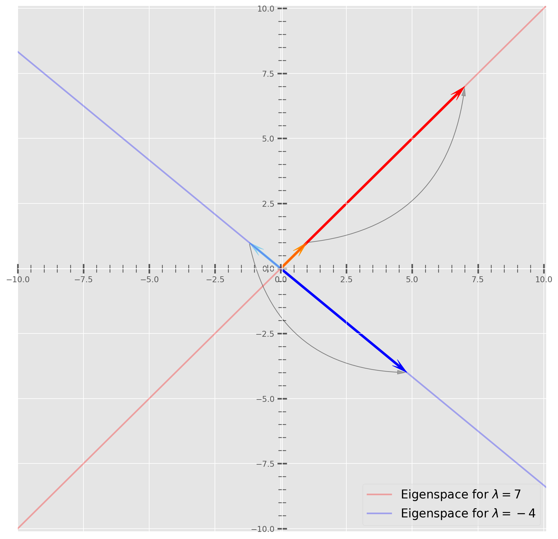
Geometric Intuition
Eigenvector has a special property that preserves the pointing direction after linear transformation.To illustrate the idea, let’s plot a ‘circle’ and arrows touching edges of circle.
Start from one arrow. If you want to draw a smoother circle, you can use parametric function rather two quadratic functions, because cicle can’t be draw with one-to-one mapping.But this is not the main issue, we will live with that.
x = np.linspace(-4, 4)
y_u = np.sqrt(16 - x**2)
y_d = -np.sqrt(16 - x**2)

fig, ax = plt.subplots(figsize=(8, 8))
ax.plot(x, y_u, color="b")
ax.plot(x, y_d, color="b")

ax.scatter(0, 0, s=100, fc="k", ec="r")

ax.arrow(
    0,
    0,
    x[5],
    y_u[5],
    head_width=0.18,
    head_length=0.27,
    length_includes_head=True,
    width=0.03,
    ec="r",
    fc="None",
)
plt.show()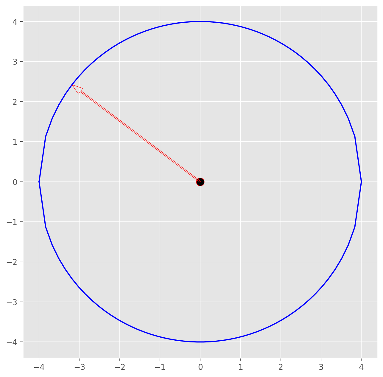
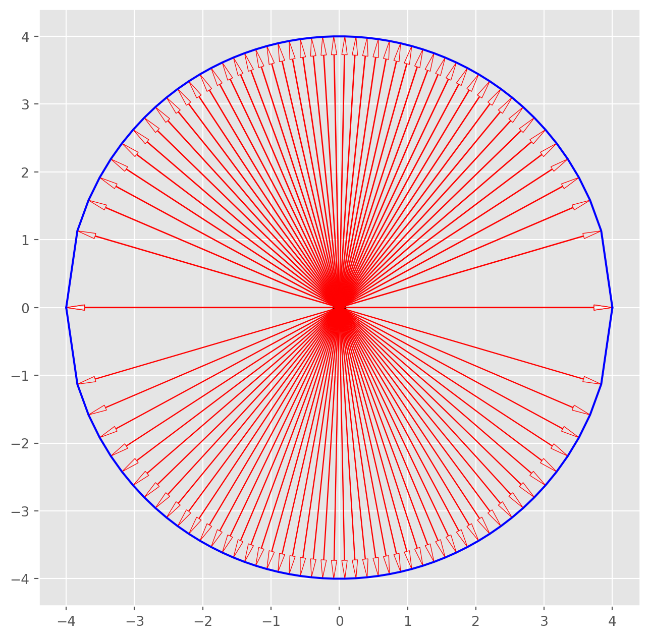
Now, the same ‘circle’, but more arrows.
x = np.linspace(-4, 4, 50)
y_u = np.sqrt(16 - x**2)
y_d = -np.sqrt(16 - x**2)

fig, ax = plt.subplots(figsize=(8, 8))
ax.plot(x, y_u, color="b")
ax.plot(x, y_d, color="b")

ax.scatter(0, 0, s=100, fc="k", ec="r")

for i in range(len(x)):
    ax.arrow(
        0,
        0,
        x[i],
        y_u[i],
        head_width=0.08,
        head_length=0.27,
        length_includes_head=True,
        width=0.01,
        ec="r",
        fc="None",
    )
    ax.arrow(
        0,
        0,
        x[i],
        y_d[i],
        head_width=0.08,
        head_length=0.27,
        length_includes_head=True,
        width=0.008,
        ec="r",
        fc="None",
    )
Now we will perform linear transformation on the circle. Technically, we can only transform the points - the arrow tip - that we specify on the circle.
We create a matrix
\[ A = \left[\begin{matrix} 3 & -2\\ 1 & 0 \end{matrix}\right] \]
Align all the coordinates into two matrices for upper and lower half respectively.
\[ V_u = \left[\begin{matrix} x_1^u & x_2^u & \ldots & x_m^u\\ y_1^u & y_2^u & \ldots & y_m^u \end{matrix}\right]\\ V_d = \left[\begin{matrix} x_1^d & x_2^d & \ldots & x_m^d\\ y_1^d & y_2^d & \ldots & y_m^d \end{matrix}\right] \]
The matrix multiplication \(AV_u\) and \(AV_d\) are linear transformation of the circle.
A = np.array([[3, -2], [1, 0]])

Vu = np.hstack((x[:, np.newaxis], y_u[:, np.newaxis]))
AV_u = A @ Vu.T

Vd = np.hstack((x[:, np.newaxis], y_d[:, np.newaxis]))
AV_d = A @ Vd.T
The circle becomes an ellipse. However, if you watch closely, you will find there are some arrows still pointing the same direction after linear transformation.
fig, ax = plt.subplots(figsize=(8, 8))

for i in range(len(x)):
    ax.arrow(
        0,
        0,
        AV_u[0, i],
        AV_u[1, i],
        head_width=0.18,
        head_length=0.27,
        length_includes_head=True,
        width=0.03,
        ec="darkorange",
        fc="None",
    )
    ax.arrow(
        0,
        0,
        AV_d[0, i],
        AV_d[1, i],
        head_width=0.18,
        head_length=0.27,
        length_includes_head=True,
        width=0.03,
        ec="darkorange",
        fc="None",
    )
ax.axis([-15, 15, -5, 5])
plt.show()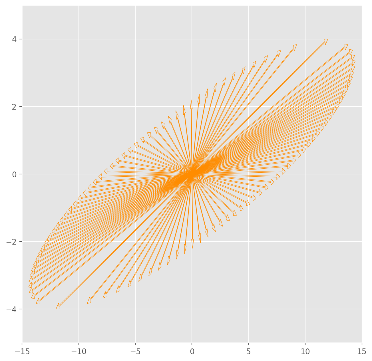
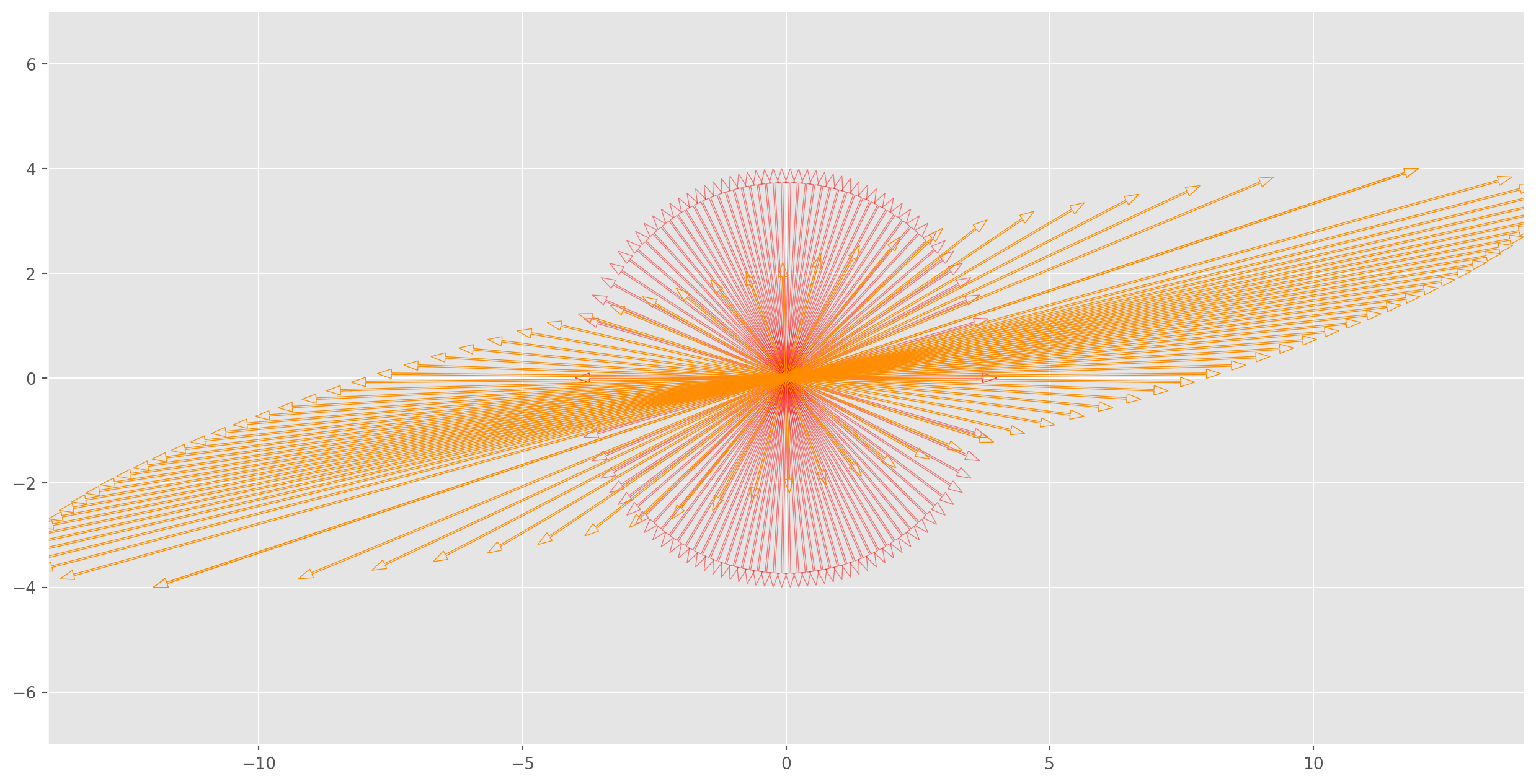
We can plot the cirle and ellipse together, those vectors pointing the same direction before and after the linear transformation are eigenvector of \(A\), eigenvalue is the length ratio between them.
k = 50
x = np.linspace(-4, 4, k)
y_u = np.sqrt(16 - x**2)
y_d = -np.sqrt(16 - x**2)

fig, ax = plt.subplots(figsize=(16, 8))

ax.scatter(0, 0, s=100, fc="k", ec="r")

for i in range(len(x)):
    ax.arrow(
        0,
        0,
        x[i],
        y_u[i],
        head_width=0.18,
        head_length=0.27,
        length_includes_head=True,
        width=0.03,
        ec="r",
        alpha=0.5,
        fc="None",
    )
    ax.arrow(
        0,
        0,
        x[i],
        y_d[i],
        head_width=0.18,
        head_length=0.27,
        length_includes_head=True,
        width=0.03,
        ec="r",
        alpha=0.5,
        fc="None",
    )

A = np.array([[3, -2], [1, 0]])

v = np.hstack((x[:, np.newaxis], y_u[:, np.newaxis]))
Av_1 = A @ v.T

v = np.hstack((x[:, np.newaxis], y_d[:, np.newaxis]))
Av_2 = A @ v.T

for i in range(len(x)):
    ax.arrow(
        0,
        0,
        Av_1[0, i],
        Av_1[1, i],
        head_width=0.18,
        head_length=0.27,
        length_includes_head=True,
        width=0.03,
        ec="darkorange",
        fc="None",
    )
    ax.arrow(
        0,
        0,
        Av_2[0, i],
        Av_2[1, i],
        head_width=0.18,
        head_length=0.27,
        length_includes_head=True,
        width=0.03,
        ec="darkorange",
        fc="None",
    )
n = 7
ax.axis([-2 * n, 2 * n, -n, n])
plt.show()